The It’s A Small World Facebook Engineering Puzzle (smallworld) is probably one of the more difficult snack-level problems; it’s also one of the funnest since the standard solution involves using a nifty data structure (note: Facebook took down the original puzzle so I’m linking to another site with the description). Even at first glance, it’s easy to understand the objective of the puzzle. The input is a list of Cartesian coordinates on a two-dimensional plane, and the goal is to find the 3 closest points for every point in the list.
In fact, this problem is commonly found in applications we all use everyday. Be it location based mobile apps, mapping software, or recommendations systems, chances are you’ve experienced the need to find things that are “close to” other things, whether physically or abstractly. Let’s dive a little deeper and see how it all works.
Now, if you think back to basic geometry, you’ll remember that the Pythagorean Theorem is handy in finding the distance between two points. For any two points A and B, we simply need to treat the line segment between A and B as the hypotenuse of a triangle. However, since we’re merely using relative distances to compare the points, the actual distance value isn’t required. Thus, we can save ourselves the cost of calculating a square root. Assuming that points are represented as 2-element arrays for the (x, y) coordinates, the distance function looks like this:
def dist(p1, p2)
  a = p1[0] - p2[0]
  b = p1[1] - p2[1]
  return (a * a) + (b * b)
end
With the ability to calculate the distance between two points, let’s shoot for the easiest, most straightforward way to solve the puzzle as a first attempt. The naive approach would be to go through the list of points, and calculate the distance between it and all other points, and keep track of the three closest points. It’s a simple solution, but runs in O(n2). There has to be a more clever way.
“O kd-tree, O kd-tree”
What if we can store the points in some sort of auxiliary data structure that would be more efficient for searching for points by proximity to a given point? That might speed things up a bit. It turns out that there’s a nifty data structure called the kd-tree that is a helpful space-partitioning data structure. A kd-tree is short for k-dimensional tree, and is a binary tree that evenly partitions a set of points at each level into two branches.
In a two-dimensional kd-tree, each level in the tree alternates between the x-axis and y-axis in order to partition the points. That is, at the root level, all the points to the left of the root point have smaller x-values, and all the points to the right have larger x-values. At one level lower, the tree partitions according to the y-value. Thus, all the points in the left branch of a node have smaller y-values, and all the points in the right branch have greater y-values. The next level splits by the x-axis, and so on.
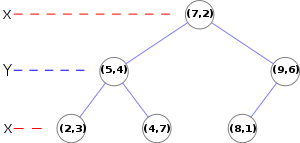
For example, a kd-tree that represents a small set of points on a Cartesian plane might look something like this (courtesy of Wikipedia):
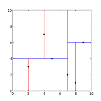
The kd-tree above represents this space partitioning:
Each colored line segment represents a branch in the tree, which effectively divides each sub-tree into two halves. At the root level, we have the point (7, 2), and the two branches divide the entire set of points into two sets: one with points to the left of (7, 2), and the other with points to the right. As you can see, each partition is further divided into halves, and the partitions match up directly with the branches in the kd-tree.
Constructing such a kd-tree is fairly straightforward. Given a list of points, we need to alternate between different the two axes as we go deeper in the tree. Once we know the axis (dimension) we’re working in, we can go through the list of points and find the median point according to its value on the axis. Here, we can actually optimize the construction algorithm by using a linear-time median selection, such as the one covered in CLRS. However, I’ve found that standard sort-then-select approach is sufficient. Once the median point has been found, it’s simply a matter of splitting the points up into two branches, and recursively processing each branch.
def build_tree(points, depth = 0)
  unless points.empty?
    axis = depth % 2
    points = points.sort { |a, b| a[axis] <=> b[axis] }
    median = points.size / 2
    return {
      :point => points[median],
      :left  => build_tree(points[0, median], depth+1),
      :right => build_tree(points[median+1, points.size],
                           depth+1),
    }
  end
end
Now that we have the locations of our friends in the small world organized in a neat little kd-tree, we need an approach that takes advantage of this data structure to efficiently find the nearest friends for each person. By now, some of you may have recognized that this problem is a k-nearest neighbor search. To keep things simple, let’s first tackle the problem of finding the single nearest neighbor for each given friend.
To find the nearest neighbor for a given point using the kd-tree we just built, we need to search through the tree in an appropriate manner. They key to the kd-tree traversal in a nearest neighbor search is in deciding on the right branch to explore. Since each branch in a kd-tree represents a space partition, the idea is to explore the partition that is closer to the point in question first. For a two-dimensional kd-tree, it’s easy to visualize this approach.
An Illustrative Example
Take the example tree from above as an example. Say we’re looking for the nearest neighbor of the point at (6, 5). We start at the root node, and see the point (7, 2), which we remember as the best candidate so far (since it’s the only one we’ve examined). At the root node, the point (7, 2) acts as a divider along the x-axis. That is, its left and right sub-trees are partitioned at x = 7. Since we’re looking for the point closest to (6, 5), we want to first explore the left partition - the left sub-tree rooted at (5, 4) - as that partition is closer.
Since the point (5, 4) is actually closer to our target than the best candidate so far, we’ll replace the candidate with (5, 4). Likewise, we’ll look at both branches, which now act as partitions on the y-axis. The right sub-tree represents the half that is closer to the target point, so we’ll examine it first. It contains (4, 7), which is not closer to our target than our best candidate. Since we’ve hit a leaf node, we stop and examine the left sub-tree.
At this point, we are exploring what is considered to be the “far” branch of the tree. By looking at our best candidate so far, we can decide whether or not the far branch is worth exploring. Conceptually, this is equivalent to drawing a circle around the target point, where the circle’s radius is equal to the distance from the target point to the best candidate point. This circle represents the “best estimate” of the target point’s nearest neighbor. If the far branch represents a partition where none of the points can possibly be closer than the best estimate so far (i.e. the best estimate circle does not intersect the partition), then we can forgo exploring the far branch altogether.
Going back to our example, since the far branch in question represents a split along the y-axis, we can actually calculate the minimum distance between any point in this branch and the target point. This split along the y-axis is at y = 4. Thus, any point in this partition must be at least 1 unit away from our target point. However, our best candidate so far, (5, 4), is actually approximately 1.41 (square root of 2) units away from the target. Thus, we should still examine this branch.
At this point, you should be able to see how the algorithm will proceed as it explores the rest of the kd-tree. In the end, the algorithm will determine that (5, 4) is in fact the closet neighbor to our target point of (6, 5). Let’s formalize this in code.
def nearest(node, point, min = node[:point], depth = 0)
  if !node.nil?
    axis = depth % 2
    d = point[axis] - node[:point][axis]

    # Determine the near and far branches
    near = d <= 0 ? node[:left] : node[:right]
    far = d <= 0 ? node[:right] : node[:left]

    # Explore the near branch
    min = nearest(near, point, min, depth + 1)

    # If necessary, explore the far branch
    if d * d < dist(point, min)
      min = nearest(far, point, min, depth + 1)
    end

    # Update the candidate if necessary
    if dist(point, node[:point]) < dist(point, min)
      min = node[:point]
    end
  end
  return min
end
Love Thy Neighbors
How do we extend the nearest neighbor search to find the nearest three neighbors? It’s actually quite easy to do, and simply requires keeping track of a bit of state. As a matter of fact, we can generalize it for finding the k-nearest neighbors. The trick is to keep track of a list of the k best candidates, instead of a single candidate. Whenever a new candidate is found, it should be inserted into the list if it is closer to the target point.
def nearest_k(node, point, k, min = [], k_dist = Float::MAX, depth = 0)
  if !node.nil?
    axis = depth % 2
    d = point[axis] - node[:point][axis]

    # Determine the near and far branches
    near = d <= 0 ? node[:left] : node[:right]
    far = d <= 0 ? node[:right] : node[:left]

    # Explore the near branch
    min, k_dist = nearest_k(near, point, k, min, k_dist, depth+1)

    # If necessary, explore the far branch
    if d * d < k_dist
      min, k_dist = nearest_k(far, point, k, min, k_dist, depth+1)
    end

    # Save the current point as a candidate if it's eligible
    d = dist(point, node[:point])
    if d < k_dist

      # Do a binary search to insert the candidate
      i, j = 0, min.size
      while i < j
        m = (i + j) / 2
        if min[m][1] < d
          i = m + 1
        else
          j = m
        end
      end
      min.insert(i, [node[:point], d])

      # Keep only the k-best candidates
      min = min[0, k]

      # Keep track of the radius of the "best estimates" circle
      k_dist = min[min.size - 1][1] if min.size >= k
    end
  end
  return min, k_dist
end
Since we’re looking for the nearest three friends for each friend in the world, we actually want to find the nearest k = 4 neighbors. By definition, each person is his or her own nearest neighbor, so we’ll need to skip the first point that we find. After we put it all together, we should be well on our way to finding ways to more efficiently visit our friends.
#!/usr/bin/ruby
friends = [
  [0.0, 0.0, 1],
  [-10.1, 10.1, 2],
  [12.2, -12.2, 3],
  [38.3, 38.3, 4],
  [179.99, 79.99, 5],
]

k = 4
tree = build_tree(friends)
friends.each do |f|
  near, d = nearest_k(tree, f, k)
  puts "#{f[2]} " + near[1, k].map { |n| n[0][2] }.join(',')
end
If you enjoyed this post, you should follow me on Twitter @cloudkj. If you’re interested in more puzzle fun, you should check out my posts about various other puzzles, such as Liar Liar, Gattaca, Dance Battle, User Bin Crash, and Refrigerator Madness.
Food For Thought
- What is the run-time complexity of the algorithm?


Comments